Source: Particle Swarm
Part 1: Given the initial position, velocity, and acceleration of a large number of particles, which particle will stay the closet to the origin as the simulation runs to infinity?
So this is actually something of a trick question. In order to answer this, you have to realize that as you go to infinity, the initial position and velocity don’t really matter at all1. The particle that has the acceleration vector with the lowest magnitude will end up the closest point to the origin after all of the points are accelerating ever more quickly away from one another.
To whit:
# PART 1
# Calculate which point is acclerating away from the origin the slowest
# Assumptions:
# - All particles will eventually move away from the origin increasingly quickly
# - The particle accelerating the slowest is the one that will eventually fall behind
# - If two have equal acceleration, the one that started closer to the origin wins

slowest_acceleration = None
slowest_distance = None
slowest_index = None

for index, point in enumerate(points):
    p, v, a = point
    acceleration = lib.vector_distance(a, origin)

    distance = lib.vector_distance(p, origin)

    new_best = (
        slowest_acceleration == None
        or acceleration < slowest_acceleration
        or (acceleration == slowest_acceleration and distance < slowest_distance)
    )

    if new_best:
        lib.log(f'New slowest acceleration point {index}: {acceleration}')

        slowest_acceleration = acceleration
        slowest_distance = distance
        slowest_index = index

print(f'{slowest_index} has the slowest acceleration ({slowest_acceleration})')
The only caveat comes up if two points happen to have the same slowest accelerating. In this case, we want whichever one started closer to the origin, since it will be that same distance closer to the origin for all time.
This also assumes that you have the points already loaded, but that’s a straight forward parsing problem. It also uses a few new library functions for vector math on tuples:
def vector_add(a, b):
    return tuple(i + j for i, j in zip(a, b))

def vector_distance(a, b):
    return sum(abs(i - j) for i, j in zip(a, b))

def vector_scale(s, a):
    return tuple(s * i for i in a)
vector_add will add two vectors together (useful for updating position from velocity or velocity from acceleration). vector_distance will return how far apart two vectors are. This can also be used to find the magnitude of a vector if either is the zero vector. vector_scale takes a vector and scales each number by a value. This is useful for running a simulation to an arbitrary distance out, for example (I don’t actually use this in my final solutions).
Part 2: Assume that the particles can collide. Once the solution reaches a steady state, how many particles are left?
This one is a bit more complicated. To do this, we do actually want to run the simulation.
First, a function that will take in the position, velocity, and acceleration of a point and return a generator that will yield each position the point will be at over time:
def simulate(p, v, a):
    '''
    Yield points along a curve until they are moving away from zero after speeding up.
    '''

    last_speed = None
    speeding_up = False

    last_distance_to_zero = None
    moving_away = False

    for tick in itertools.count():
        yield p

        v = lib.vector_add(v, a)
        p = lib.vector_add(p, v)
I like generators. They make for elegant code.
Next, we use that to create a generator for every point in the simulation. We advance each one tick at a time (so they stay in sync) and check for any collisions:
# PART 2
# Calculate how many points are left after collisions
# Assumptions:
# - Stop if all particles are moving apart (maximum pairwise distance is increasing)
#   (Technically you also have to know that all particles are currently accelerating)

simulators = [simulate(*point) for point in points]
last_max_distance = None

for tick in itertools.count():
    current_points = [next(simulator) for simulator in simulators]

    # Remove any particles that have collided

    to_remove = {
        i
        for i, pa in enumerate(current_points)
        for j, pb in enumerate(current_points)
        if i != j and pa == pb
    }

    if to_remove:
        lib.log(f'{list(to_remove)} collided on tick {tick}')

    simulators = [
        simulator
        for index, simulator in enumerate(simulators)
        if index not in to_remove
    ]

    # Check if everything is moving apart (we can stop then)

    max_distance = max(
        lib.vector_distance(p1, p2)
        for p1 in current_points
        for p2 in current_points
    )

    lib.log(f'Maximum distance: {max_distance} (last: {last_max_distance})')

    if last_max_distance:
        if max_distance > last_max_distance:
            break
    else:
        last_max_distance = max_distance

print(f'{len(simulators)} left after collisions')
The main assumption here is that as the simulation runs to infinity, we’ll eventually get to a point where all the particles are moving ever more quickly apart from each other. This could have a problem if we ever have an earlier tick where the particles happen to be moving apart before they all hit their inflection points, but it turns out that at least in the input I was given (and probably most of them), this is a perfectly safe approximation to make.
Once you’ve stopped the simulation at this point, you know how far apart all of the particles were.
One thing that I would like to see is just what this simulation looks like. I know the particles will start in a rough ball which will likely contract and then blow apart, but it would still be interesting to see it. The main problem comes with rendering the points in 3D space. Let’s
To do this, we will inject a rendering function after we’ve made each simulation step to render each frame as a PNG:
lib.add_argument('--render', action = 'store_true', help = 'On part 2, render each frame as an image')
lib.add_argument('--render-frames', type = int, default = -1, help = 'If specified, render this many frames rather than stopping when we have an answer')
lib.add_argument('--render-region', type = int, default = 15000, help = 'The maximum x/y/z coordinate to render for --render-frames')

if lib.param('render'):
    import matplotlib.pyplot as plt
    from mpl_toolkits.mplot3d import Axes3D

    fig = plt.figure()

    render_region = lib.param('render_region')
    ax = fig.add_subplot(111, projection = '3d')
    ax.set_xlim([-render_region, render_region])
    ax.set_ylim([-render_region, render_region])
    ax.set_zlim([-render_region, render_region])

    ax.scatter(*zip(*current_points))

    fig.savefig(f'frame-{tick:04d}.png')

    # If we want to limit the number of frames to render and we've hit that, stop
    if 0 < lib.param('render_frames') <= tick:
        break
One neat trick there is that we’re taking current_points and using zip(*current_points) to unpack that into three parameters: xs, ys, zs (a list of x, y, and z coordinates) which we are then passing as the first three arguments to scatter. This will render frames like this:
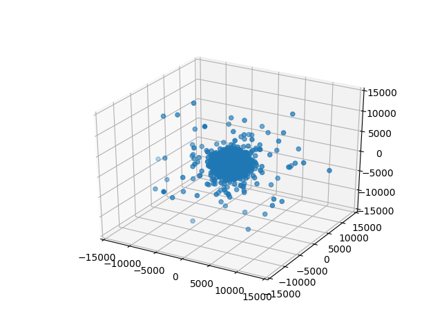
frame-0000.png
We can combine these with ImageMagick:
$ convert -delay 10 frame-*.png simulation.gif
You may have noticed that I set a limit on the axes with set_xlim etc. This is so that the bounds are automatically calculated per frame. That’s what I did originally and they jumped around rather a lot. This works better.
Plus, watching them blow past the specified bounds is kind of hilarious.
If we’re running it all without rendering frames, it’s more or less quick enough (especially since it’s for both parts2):
$ python3 run-all.py day-20

day-20  python3 miniature-universe-simulator.py input.txt       70.74992203712463       243 has the slowest acceleration (2); 648 left after collisions