I was playing with image library and started to think about more ways that I could generate images. One idea that came to mind was to generate a bunch of colored points on the image and then color every other pixel based on which seed point was closest. Turns out, that’s exactly what a Voronoi diagramis… The Wikipedia article at least says that Voronoi diagrams can be traced back at least to Descartesin 1644, so I guess at least I’m in good company. 😄

Anyways, the code is actually really simple, given the (c211 image) library’s make-image function:

; fill an rs x cs by coloring each point based on:
; the color in cls associated with the closest point in pts
; calculate all of the distances, sort for smallest, use that one
(define (fill dist rs cs pts cls)
  (make-image rs cs
    (lambda (r c)
      (cadar
        (sort
          (lambda (pc1 pc2) (< (car pc1) (car pc2)))
          (map (lambda (pt cl)
                 (list
                       (dist (list r c) pt) cl)) pts cls))))))

Yeah. That’s it. It’s a little more complicated as you need to give it a distance function. Here’s the boring everyday distance function that you’re probably familiar with:

; distance function
(define (distance p1 p2)
  (expt (+ (expt (- (car p1) (car p2)) 2)
           (expt (- (cadr p1) (cadr p2)) 2))
    0.5))

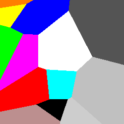
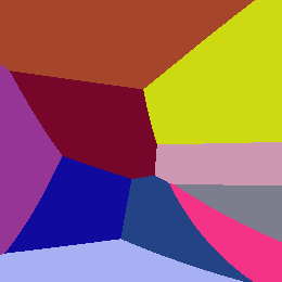
And if you generate a random collection of starting points and colors, you might a Voronoi diagram that looks an awful lot like this one:

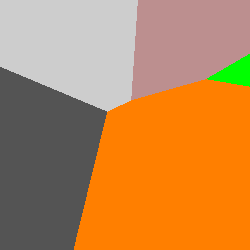
But what’s really interesting (at least to me) is when you start using different distance functions. For example, if you instead use Manhattan / taxicab distance (with the same points), you get something more like this:

; manhattan distance function
(define (manhattan p1 p2)
  (+ (abs (- (car p1) (car p2))) (abs (- (cadr p1) (cadr p2)))))

Basically, you get a lot more straight lines at 45 and 90 intervals rather than the more varied angles in the original.

As another function, what if you take the standard distance function but rather than squaring and then taking the square root, you use fourth powers:

; take a quartic instead of a square
(define (quartic p1 p2)
  (expt (+ (expt (- (car p1) (car p2)) 4)
           (expt (- (cadr p1) (cadr p2)) 4))
    0.25))

Same sort of thing as the original distance function, but you get a little more bowing and curving than the straight distance allows. Mostly out of curiosity, I’ll leave it as an exercise for why I jumped from 2nd powers to 4th. It turns out that odd powers do strange things to signs. 😄

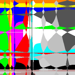
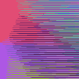
Finally, what if you invert the distance function with a simple 1/n? Or perhaps you just negate the distance function, weighting points further rather than closer. You might get something like this (with the /0 function designed to ignore dividing by 0):

; a very special division that can divide by 0 😄
(define (/0 a b) (if (= b 0) 1e9 (/ a b)))

; use some strange negative power
(define (inverse p1 p2)
  (+ (/0 1 (abs (- (car p1) (car p2)))) (/0 1 (abs (- (cadr p1) (cadr p2))))))

; negative distance
(define (ndist p1 p2)
  (- (distance p1 p2)))

Now rather than choosing the closet point, you’re essentially choosing the furthest. It gets a little more complicated if the fraction you’re dealing with is under 1, but since we’re dealing with whole numbers of pixels that really didn’t come up.

Or what if you do something similar to Manhattan distance function, but instead of adding the two, you multiply them? What if you just take the bigger of the two? The smaller?

; multiply the differences
(define (mul/min/max-xy p1 p2)
  (*/min/max (abs (- (car p1) (car p2))) (abs (- (cadr p1) (cadr p2)))))

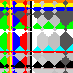
All sorts of interesting patterns there when the minimum (or the dominant factor in a multiplication) switches from one axis to the other. Neat stuff.

Anyways, does anyone have a different distance function that does something interesting? Feel free to leave a comment below. You can either generate the images yourself in Wombat or just leave the code and I’ll run it for you.

If you’d like to download the source code, you can do so here: voronoi source

Update: Here are the images reference in my comment below:

• Using the original algorithm:
  

  

• Using normalized coordinates:
  

  

Update: For the second comment (working in degrees), I actually rewrote the code to work in Racket, since I’m far more familiar with that:

(require images/flomap)

(struct pt (x y))
(struct cpt pt (c))

(define (voronoi width height distance seeds)
  (flomap->bitmap
   (build-flomap*
    3 width height
    (λ (x y)
      (call-with-values
       (thunk
        (for/fold ([min-distance +inf.0] [min-color #f])
                  ([seed (in-list seeds)])
          (define new-distance (distance (pt x y) seed))
          (if (< new-distance min-distance)
              (values new-distance (cpt-c seed))
              (values min-distance min-color))))
       (λ (distance color) color))))))

(define (random-seeds width height count)
  (for/list ([i (in-range count)])
    (cpt (random width) (random height)
         (vector (random) (random) (random)))))

That lets us translate your new function fairly easily (although the offsets are a little interesting):

(voronoi
 160 40
 (λ (pt1 pt2)
   ; Unpack points
   (match-define (pt x1^ y1^) pt1)
   (match-define (pt x2^ y2^) pt2)

   ; Rescale to the range [20, 80] and [40, 80]
   (define x1 (+ x1^ 20))
   (define y1 (+ y1^ 40))
   (define x2 (+ x2^ 20))
   (define y2 (+ y2^ 40))

   (sqrt (+ (sqr (- (* x1 (cos (degrees->radians y1)))
                    (* x2 (cos (degrees->radians y2)))))
            (sqr (- y1 y2)))))

 (random-seeds 160 40 10))

Here are a few examples:

That’s really cool. They sort of look like scales!

If you relax the range and let it go a full circle (x and y both ranging from 0 to 360), you get this:

Not quite scales any more, but there is a lot of neat structure in there.